Authors:
(1) Maggie D. Bailey, Colorado School of Mines and National Renewable Energy Lab;
(2) Douglas Nychka, Colorado School of Mines;
(3) Manajit Sengupta, National Renewable Energy Lab;
(4) Aron Habte, National Renewable Energy Lab;
(5) Yu Xie, National Renewable Energy Lab;
(6) Soutir Bandyopadhyay, Colorado School of Mines.
Table of Links
Bayesian Hierarchical Model (BHM)
Appendix B: Regridding Coefficient Estimates
5 Results
The results presented here summarize the metrics outlined in Sect. 4. As the true coefficients are not known, we have supplemented the analysis with a simulation study. The design and results for this study are described in given in Appendix A.
5.1 Posterior Distribution of Model Coefficients
Resulting parameter estimates from the posterior distribution vary by location and coefficient. Here we will refer to parameter bias as the difference between the naive estimate and that based on the Bayesian analysis. In general, the naive regridding model coefficient estimates are within the 95% credible intervals of the posterior distributions for the respective coefficient. An example of the distributions compared to the naive regridding estimate can be seen in Figure 2 for a location near the coastline of California across four different months. The green lines represent the naive regridding method and the purple the Bayesian regridding method. In general, there is strong agreement between the two methods in both the point or median coefficient estimate as well as the confidence or credible intervals suggesting that incorporating the uncertainty associated with the regridding step has little effect on model estimates. However, in the month of August (bottom left plot) we see a case for the WRF coefficient where the methods do not agree and this bias is off-set by the intercept estimate. This bias in the WRF coefficient was seen across many locations for the month of August.
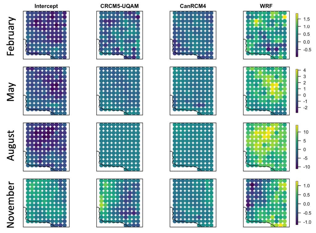
For the entire area considered, the average bias by location is shown in Figure 3. The bias is calculated as the BHM estimate subtracted from the naive regridding estimate. Values close to zero indicate little difference between the two methods. Negative values indicate that the BHM is giving a stronger weight to the model. The spatial patterns of the bias are most pronounced for the month of November and also large for the month of August. In November, the average bias between the CRCM5-UQAM and WRF coefficient are spatially opposite in their signs but both hover around zero. Here, we can see that the naive method and BHM most disagree for the WRF coefficient in the month of August, with the naive method resulting in a much higher weight for WRF compared to the BHM. For additional reference, the estimated coefficient estimates and standard errors are provided in Appendix B.
5.2 Prediction Coverage and Error Comparison
The prediction coverage of the naive regridding is calculated as the percentage of observations that are within the prediction intervals of the linear model. This is calculated by location for each of the four months considered. A similar method is implemented to calculate the coverage resulting from the BHM. We show results for the fourth months in Figure 4. Note that in the figure shown, the percent coverage reported is an average for holding out each year and shown as the difference from the nominal level of 0.95. We see similar results for the out of sample coverage compared to the naive regridding.
Similarly, the RMSE between the predicted GHI and the true GHI is lower across the study domain for August than it is for November in both the naive regridding model and the BHM, indicating better predictions for the summer month over the winter month. This is shown in Figure 5. This finding may reflect a characteristic of seasonal solar radiation. Incoming solar radiation during summer months typically has lower standard deviation when considered on a monthly or seasonal basis than
Figure 2. Posterior predictions for each coefficient compared to the naive regridding estimates for a particular location in California for February, May, August, and November (1998-2009). The solid dots represent the point estimate for the naive regridding method and the median value of posterior distribution from the Bayesian method. The whiskers represent the 95% credible and confidence intervals for the posterior distribution and the naive regridding estimates, respectively


in winter in California, indicating that there is less variability in day types (i.e. cloudy versus sunny) or amount of incoming solar radiation during the summer compared to the winter. Therefore, it makes sense that predictions have a lower RMSE in the summer months as the covariables and response have less variability during that season. The RMSE values are also lower for the naive regridding than they are for the BHM across the four months shown. When regridding uncertainty is taken into account, the predicted GHI values have a higher error than when prediction is done directly without considering regridding uncertainty. This is an interesting finding in that it suggests doing prediction directly without considering any uncertainty may produce more accurate point predictions but regridding uncertainty contributes additional variability to the final point estimates as seen in the BHM.
Figure 3. Average bias by location between the naive regridding estimate and the median of all posterior distributions for February, May, August, and November, top to bottom, respectively.

This paper is available on arxiv under CC 4.0 license.